Topology Analysis
The compute_topomesh_property method provides ways to store advanced topological features of a PropertyTopomesh as wisp properties. This avoids unnecessary re-computations of topological relationships that are not diirectly encoded in the structure, and allows powerful global computations, making advantage of the NumPy encoding of the properties.
Basic topological properties
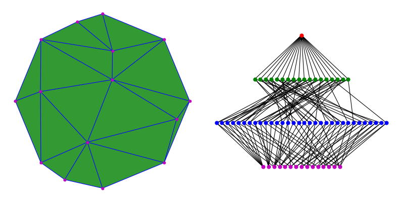
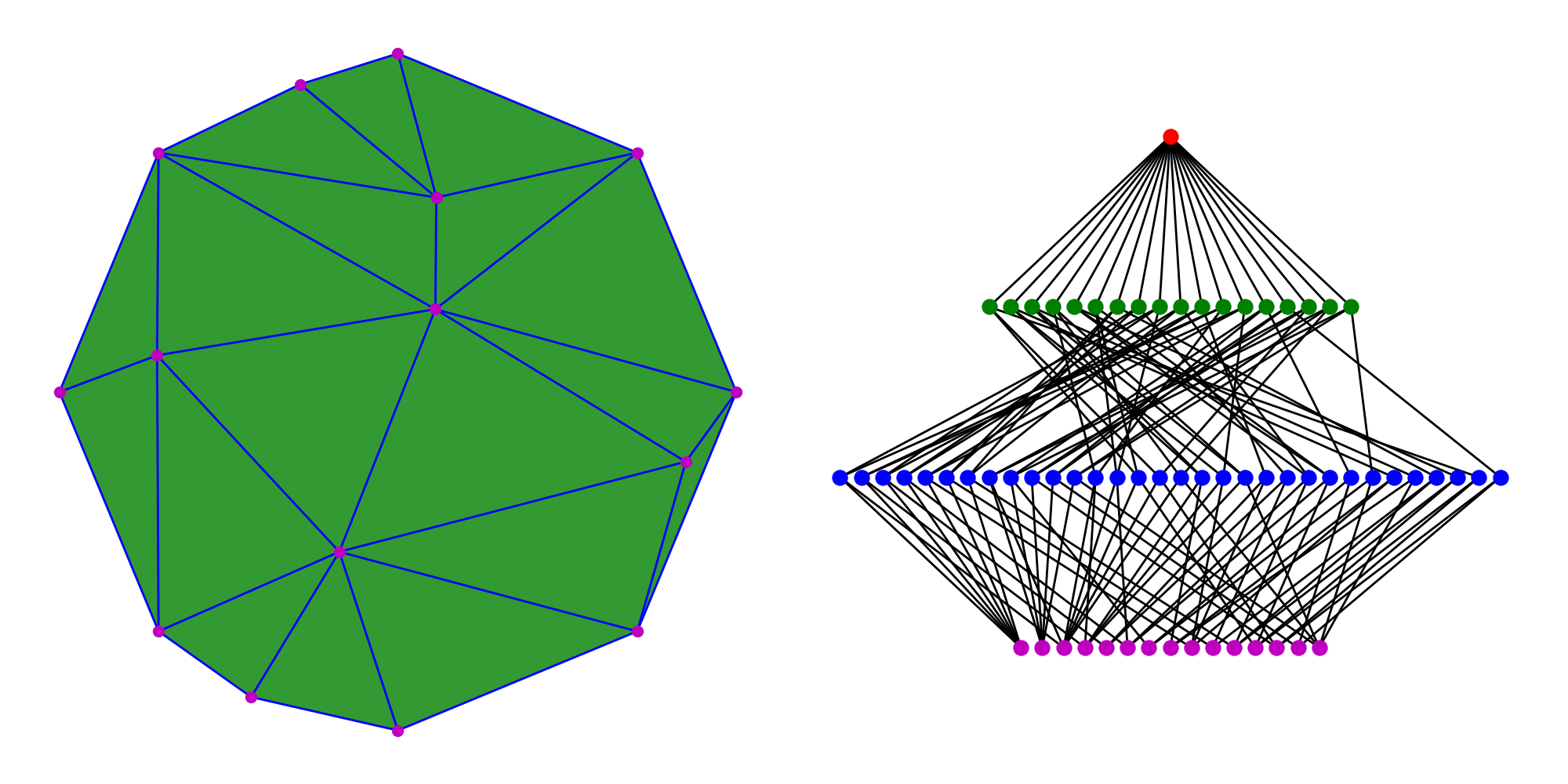
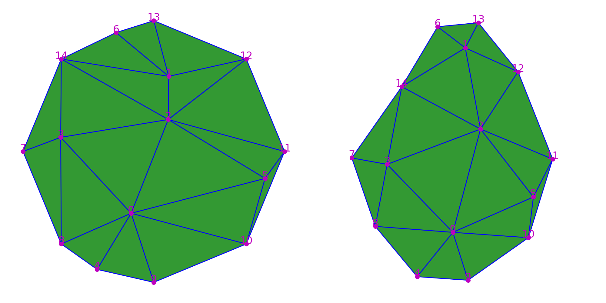
Let’s consider a rather simple triangular mesh represented by a PropertyTopomesh, here generated as a random triangulation inscribed within a circle. The only information that is stored in memory is the incidence graph displayed on the right, that is already somewhat complex.
1 2 3 | from cellcomplex.property_topomesh.example_topomesh import circle_voronoi_topomesh
_,topomesh = circle_voronoi_topomesh(2,circle_size=8,return_triangulation=True)
|
(Source code, png, hires.png, pdf)

This kind of combinatorial structure can be very costly to manipulate in Python as traversals might involve several embedded for() loops. The philosophy behind CellComplex is to give the possibility to perform computations as globally as possible, by providing tools to investigate the structure through NumPy arrays. For instance, the compute_topomesh_property offers the possibility to access the essence of the topological structure (the borders() and regions() relationships) as array properties.
1 2 3 4 | from cellcomplex.property_topomesh.analysis import compute_topomesh_property
compute_topomesh_property(topomesh,'borders',1)
print("Edge borders: "+str(topomesh.wisp_property('borders',1).values()))
|
Edge borders:   [[ 0  2]
                 [ 0  3]
                 [ 0  4]
                 [ 0  5]
                 [ 0  8]
                 [ 0  9]
                 [ 0 10]
                 [ 1  2]
                 [ 1  6]
                 [ 1 12]
                 [ 1 13]
                 [ 1 14]
                 [ 2  3]
                 [ 2  5]
                 [ 2 11]
                 [ 2 12]
                 [ 2 14]
                 [ 3  7]
                 [ 8  3]
                 [ 3 14]
                 [ 8  4]
                 [ 9  4]
                 [10  5]
                 [11  5]
                 [13  6]
                 [ 6 14]
                 [ 8  7]
                 [14  7]
                 [ 9 10]
                 [10 11]
                 [11 12]
                 [12 13]]
The main advantage of accessing data this way is the possibility to combine arrays of properties in order to make fast computations. For instance, to compute the length of all edges requires computing the norm of the difference of positions ('barycenter' property) of the edge borders, which can be written in a very condensed and efficient way in NumPy.
1 2 3 4 | edge_borders = topomesh.wisp_property('borders',1).values()
edge_border_positions = topomesh.wisp_property('barycenter',0).values(edge_borders)
edge_lengths = np.linalg.norm(np.diff(edge_border_positions,axis=1)[:,0],axis=1)
print("Edge lengths: "+str(edge_lengths))
|
Edge lengths: [1.54168209 1.58307211 1.00382853 2.11521433 1.16696402 1.1110798
               1.82197209 0.65995687 1.04620625 1.21589874 0.88074694 1.6630285
               1.66661489 1.73242215 1.84463235 1.50941624 1.87907293 0.61652321
               1.63064711 1.19783225 0.6710141  0.88910546 1.04256369 0.5089403
               0.60474705 0.9297893  1.53073373 1.53073373 1.53073373 1.53073373
               1.53073373 1.53073373]
A more usual way to perform the same computation would have been to iterate over the mesh edges using the wisps method and then to use the borders method to access each edge’s vertices, to look for their value for the barycenter property, before computing the norm. Running a computational time evaluation on such simple example already reveals the interest to manipulate the topological structure as arrays when possible, and to store low-level information (that may not appear costly to compute at first, but is systematically used) as a ready-to-use array. Especially when the computations are to be repeated, as we see that the time gain is more than 3x if we don’t need to perform the initial property storage.
1 2 3 4 5 6 7 8 9 10 11 12 13 14 15 16 17 18 19 20 21 22 | from time import time
start_time = time()
edge_border_positions = []
for e in topomesh.wisps(1):
edge_borders = list(topomesh.borders(1,e))
edge_border_positions.append([topomesh.wisp_property('barycenter',0)[v] for v in edge_borders])
edge_lengths = np.linalg.norm(np.diff(edge_border_positions,axis=1)[:,0],axis=1)
print("Loop-based computation (everytime): "+str(np.round(1000.*(time()-start_time),2))+"ms")
start_time = time()
compute_topomesh_property(topomesh,'borders',1)
edge_borders = topomesh.wisp_property('borders',1).values()
edge_border_positions = topomesh.wisp_property('barycenter',0).values(edge_borders)
edge_lengths = np.linalg.norm(np.diff(edge_border_positions,axis=1)[:,0],axis=1)
print("NumPy computation (1st time): "+str(np.round(1000.*(time()-start_time),2))+"ms")
start_time = time()
edge_borders = topomesh.wisp_property('borders',1).values()
edge_border_positions = topomesh.wisp_property('barycenter',0).values(edge_borders)
edge_lengths = np.linalg.norm(np.diff(edge_border_positions,axis=1)[:,0],axis=1)
print("NumPy computation (next time(s)): "+str(np.round(1000.*(time()-start_time),2))+"ms")
|
Loop-based computation (everytime): 0.84ms
NumPy computation (1st time): 0.59ms
NumPy computation (next time(s)): 0.22ms
Complex topology as properties
As we saw, when performing computationally heavy tasks the recommended way to manipulate a PropertyTopomesh is through the use of properties that reflect its topology. This is particularly true when the same computation has to be performed iteratively on a structure with a fixed topology, for instance whenever geometry is evolving and geometrical values need to be updated regularly. To be more efficient in this situation, the compute_topomesh_property gives access to other topological relationships that are not simply the boundary relationship between elements. Indirect relationships such as neighbor relationships, or incidence between more than one dimension (the vertices of a face typically) can be stored once as a property and a re-used to perform advanced computations.
1 2 | compute_topomesh_property(topomesh,'vertices',2)
print("Face vertices: "+str(topomesh.wisp_property('vertices',2).values()))
|
Face vertices:  [[ 0  2  9]
                 [ 0  4  9]
                 [ 5 11 12]
                 [ 0  4  5]
                 [ 6 12 13]
                 [ 0  5  6]
                 [ 5  6 12]
                 [ 2  7  8]
                 [ 2  8  9]
                 [ 1  7 14]
                 [ 1  2  7]
                 [ 0  1  2]
                 [ 0  1  6]
                 [ 1 13 14]
                 [ 1  6 13]
                 [ 4  9 10]
                 [ 3  4 10]
                 [ 3  5 11]
                 [ 3  4  5]]
In the following we will make use of these topological properties to perform a rather complex task: apply an iterative smoothing algorithm to the mesh geometry. The algorithm is a Laplacian smoothing algorithm, where the vertices are iteratively shifted towards the barycenter of their neighbors, but with a rather small coefficient. As the process will not affect the topology of the complex but only its geometry, we can compute the neighbors property on the vertices and store it in a NumPy array.
1 2 3 | compute_topomesh_property(topomesh,'neighbors',0)
print(topomesh.wisp_property('neighbors',0))
vertex_neighbors = topomesh.wisp_property('neighbors',0).values()
|
{0:  [ 2   3   4   5   8   9  10]
 1:  [ 2   6  12  13  14]
 2:  [ 0   1   3   5  11  12  14]
 3:  [ 0   2   7   8  14]
 4:  [ 0   8   9]
 5:  [ 0   2  10  11]
 6:  [ 1  13  14]
 7:  [ 3   8  14]
 8:  [ 0   3   4   7]
 9:  [ 0   4  10]
 10: [ 0   5   9  11]
 11: [ 2   5  10  12]
 12: [ 1   2  11  13]
 13: [ 1   6  12]
 14: [ 1   2   3   6   7]}
Then to estimate the center of any vertex neighborhood, we will use the barycenter property on vertices that stores their 3d position, and apply the NumPy mean function to average positions of the neighbor vertices.
1 2 | vertex_neighbor_positions = topomesh.wisp_property('barycenter',0).values(vertex_neighbors)
vertex_neighbor_center = np.array([np.mean(p,axis=0) for p in vertex_neighbor_positions])
|
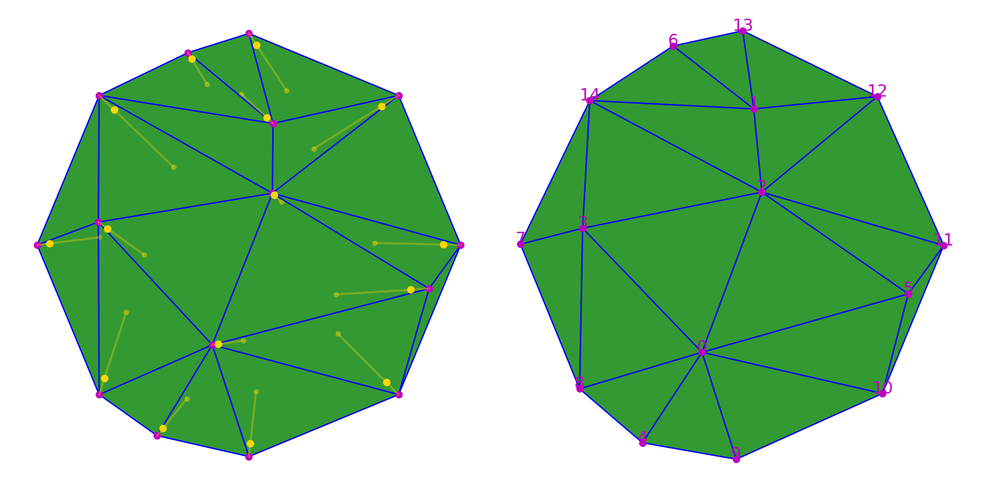
The next step is to compute a new position for all the vertices by adding to the current position a vector in the towards the neighborhood center. The vector is multiplied by a small coefficient to ensure the stability of the process. Once computed, the new positions can be affected to the vertices as barycenter property through the update_wisp_property method.
1 2 3 4 5 | coef = 0.2
vertex_positions = topomesh.wisp_property('barycenter',0).values()
new_vertex_positions = vertex_positions + 0.33*(vertex_neighbor_center-vertex_positions)
topomesh.update_wisp_property('barycenter',0,new_vertex_positions)
|
(Source code, png, hires.png, pdf)
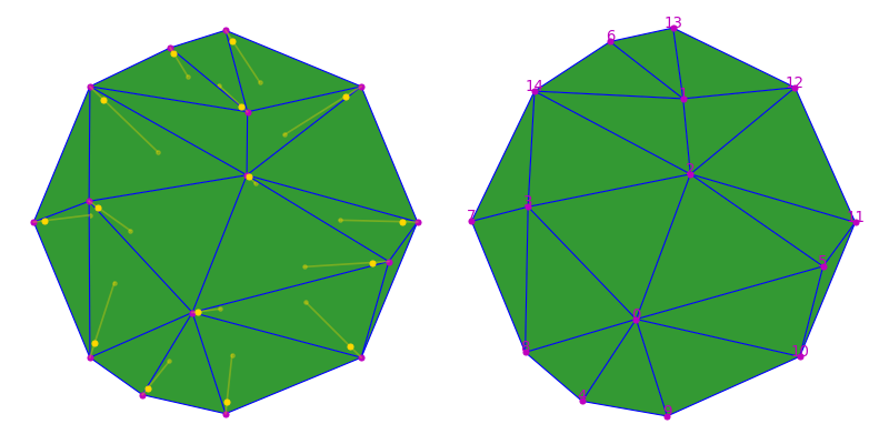
The only thiing left to do is to iterate over this position update loop to perform an interative smoothing of the initial mesh.
1 2 3 4 5 6 7 8 9 | coef = 0.2
for iteration in range(10):
vertex_positions = topomesh.wisp_property('barycenter',0).values()
vertex_neighbor_positions =  topomesh.wisp_property('barycenter',0).values(vertex_neighbors)
vertex_neighbor_center = np.array([np.mean(p,axis=0) for p in vertex_neighbor_positions])
new_vertex_positions = vertex_positions + coef*(vertex_neighbor_center-vertex_positions)
topomesh.update_wisp_property('barycenter',0,new_vertex_positions)
|
(Source code, png, hires.png, pdf)

The result of the smoothing is a global regularization of the shapes of the mesh triangles that less elongated than in the initial configuration, at the expense of the overall shape of the mesh. The use of topological properties in this case allows to write the process at a very high level and avoids going into multiple imbricated loops to obtain the same result. Most of the code in CellComplex makes use of this powerful tool for manipulating the structure, notably all the geometrical analysis tools described in Geometry Analysis.
Computable topological properties
A list of topological properties that can be passed as property_name argument to the function compute_topomesh_property, along with the wisp dimension for which they can be computed:
property_name |
0 |
1 |
2 |
3 |
type |
|---|---|---|---|---|---|
|
x |
x |
x |
list |
|
|
x |
x |
x |
list |
|
|
x |
x |
x |
x |
list |
|
x |
x |
x |
x |
list |
|
x |
x |
x |
x |
list |
|
x |
x |
x |
x |
list |