PropertyTopomesh Data Structure
The central data structure in CellComplex is a representation of cellular complexes implemented as incidence graphs, in an class called PropertyTopomesh. Cell complexes are seen as boundary representations consisting of a collection of topological elements of dimension 0 up to 3, where each higher-dimension element is defined by the set of its lower-dimension boundary elements. In PropertyTopomesh those elements are called wisps.
A
wispof dimension 0 is a vertex, and, as the lowest possible dimension, it is the only one without boundaries.
Note
Instead it is defined by its spatial position, that is generally sufficient for the geometrical embedding of the whole cellular complex.
A
wispof dimension 1 is an edge and is generally defined by exactly 2 boundary vertices.Wispsof dimension 2 are faces and require at least 3 boundary edges. If all faces have exactly 3 edges, thePropertyTopomeshforms a triangular mesh.Finally, cells correspond to the
wispsof dimension 3.
Note
Even though they conceptually represent entities of geometrical dimension 3, in a number of cases where the complex is a 2-manifold, cells may be defined as sets of faces.
Wisps : a pre-built example
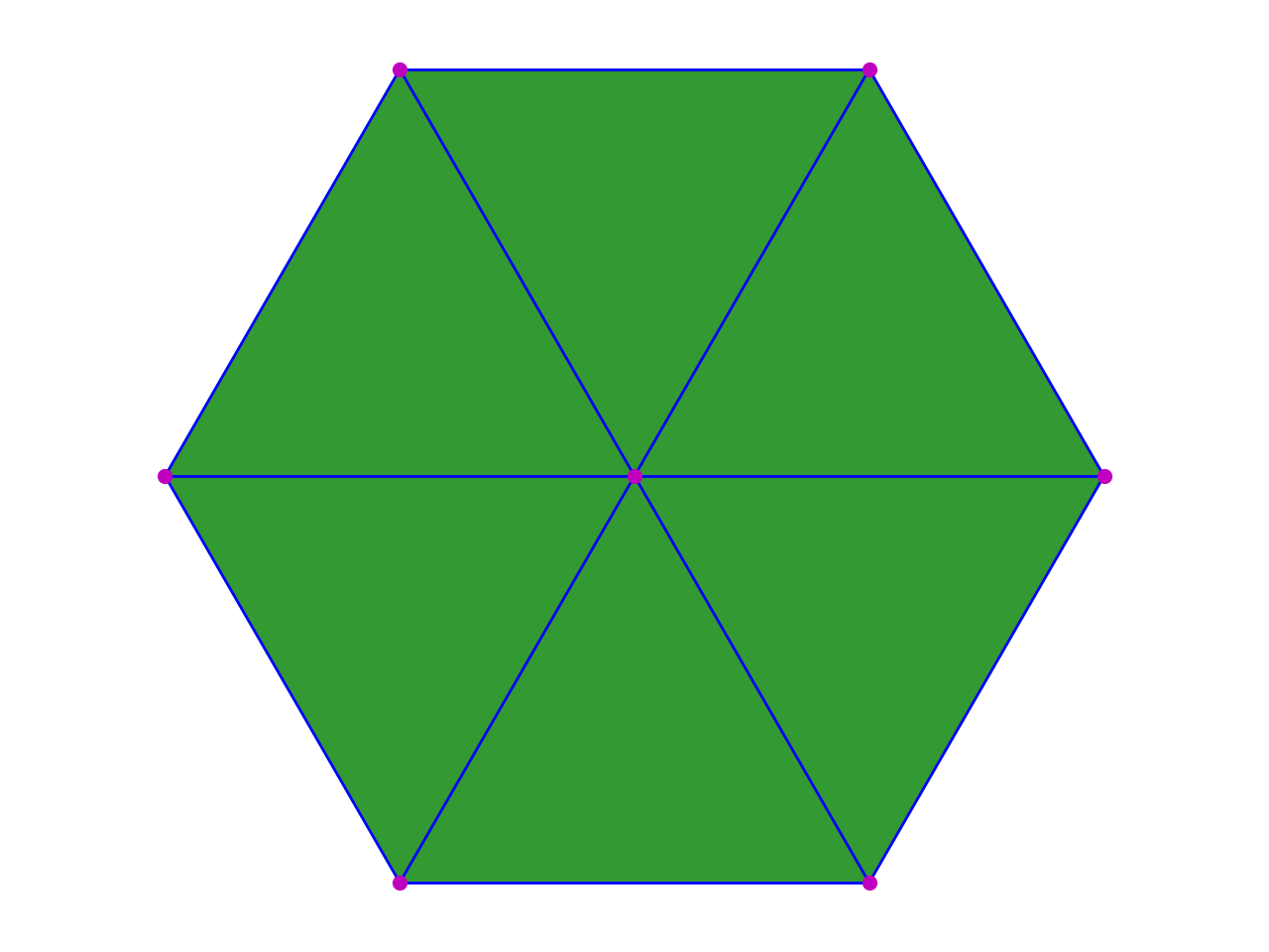
The hexagon_topomesh function creates a simple 2D-embedded cellcomplex, consisting of one hexagonal cell represented as a triangular mesh.
1 2 3 | from cellcomplex.property_topomesh.example_topomesh import hexagon_topomesh
topomesh = hexagon_topomesh()
|
(Source code, png, hires.png, pdf)
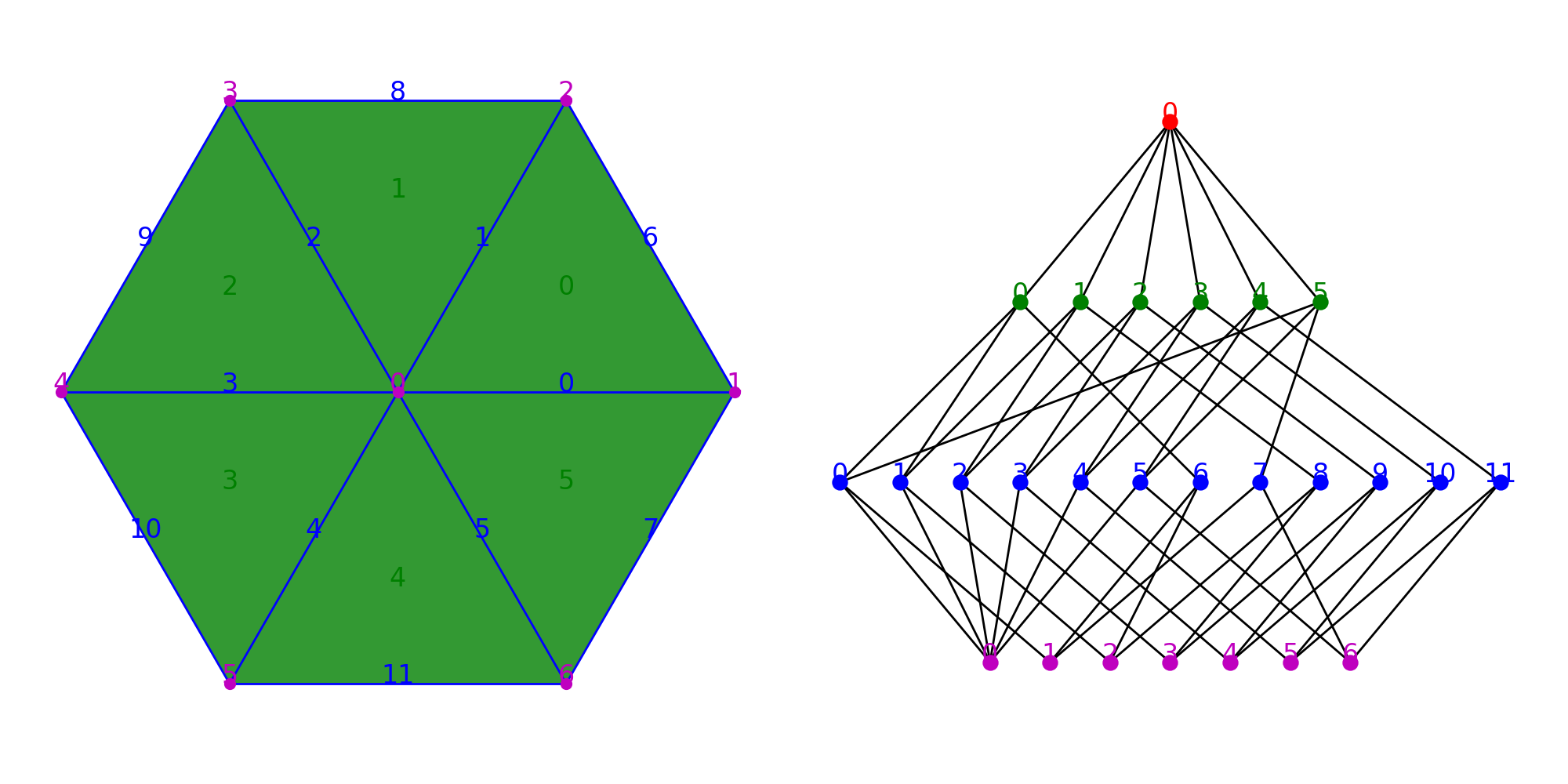
In a PropertyTopomesh, wisps are represented by unique integer IDs at each dimension. The methods nb_wisps and wisps allow to access respectively the number of elements and the list of their IDs at each dimension.
1 2 3 4 | print(topomesh.nb_wisps(0),"Vertices :",list(topomesh.wisps(0)))
print(topomesh.nb_wisps(1),"Edges :",list(topomesh.wisps(1)))
print(topomesh.nb_wisps(2),"Faces :",list(topomesh.wisps(2)))
print(topomesh.nb_wisps(3),"Cells :",list(topomesh.wisps(3)))
|
7 Vertices : [0, 1, 2, 3, 4, 5, 6]
12 Edges : [0, 1, 2, 3, 4, 5, 6, 7, 8, 9, 10, 11]
6 Faces : [0, 1, 2, 3, 4, 5]
1 Cells : [0]
The whole topology of the complex relies on the boundary relationships between its wisps. The topology relationships can be displayed as a graph showing the incidence (edges) between wisps (vertices) of contiguous dimensions.
(Source code, png, hires.png, pdf)
The whole geometry of the complex is then determined only by the spatial position assigned to each wisp of dimension 0. It is defined as a Python dictionary pairing each ID of a wisp of dimension 0 to a NumPy array representing a point in a 3-dimensional space. This dictionary is stored within the data structure as a property defined on the dimension 0, named 'barycenter'.
1 | print(topomesh.wisp_property('barycenter',0))
|
{0: [0. 0. 0. ],
1: [1. 0. 0. ],
2: [0.5 0.8660254 0. ],
3: [-0.5 0.8660254 0. ],
4: [-1. 0. 0 ],
5: [-0.5 -0.8660254 0. ],
6: [ 0.5 -0.8660254 0. ]}
Note
The property is not an instance of dict, but uses a custom implementation based on NumPy arrays called array_dict.
Link, borders and regions
In this section, we will see how to create a cell complex from scratch by defining explicitly all the boundary relationships between the topological elements.
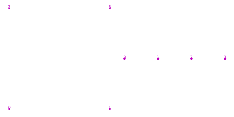
When a PropertyTopomesh is created, it comes as an empty structure containing no wisp of any dimension. The first step consists then in adding new elements using the add_wisp function, that takes a dimension and an optional ID argument. In any case the ID of the new element is returned. Then in the case of vertices, it is necessary to assign a 'barycenter' property to the newly created wisps.
1 2 3 4 5 6 7 8 | from cellcomplex.property_topomesh import PropertyTopomesh
topomesh = PropertyTopomesh()
topomesh.add_wisp(0,0)
topomesh.add_wisp(0,1)
topomesh.add_wisp(0,2)
topomesh.add_wisp(0,3)
topomesh.update_wisp_property('barycenter',0,{0:[-1,-1,0],1:[1,-1,0],2:[-1,1,0],3:[1,1,0]})
|
(Source code, png, hires.png, pdf)

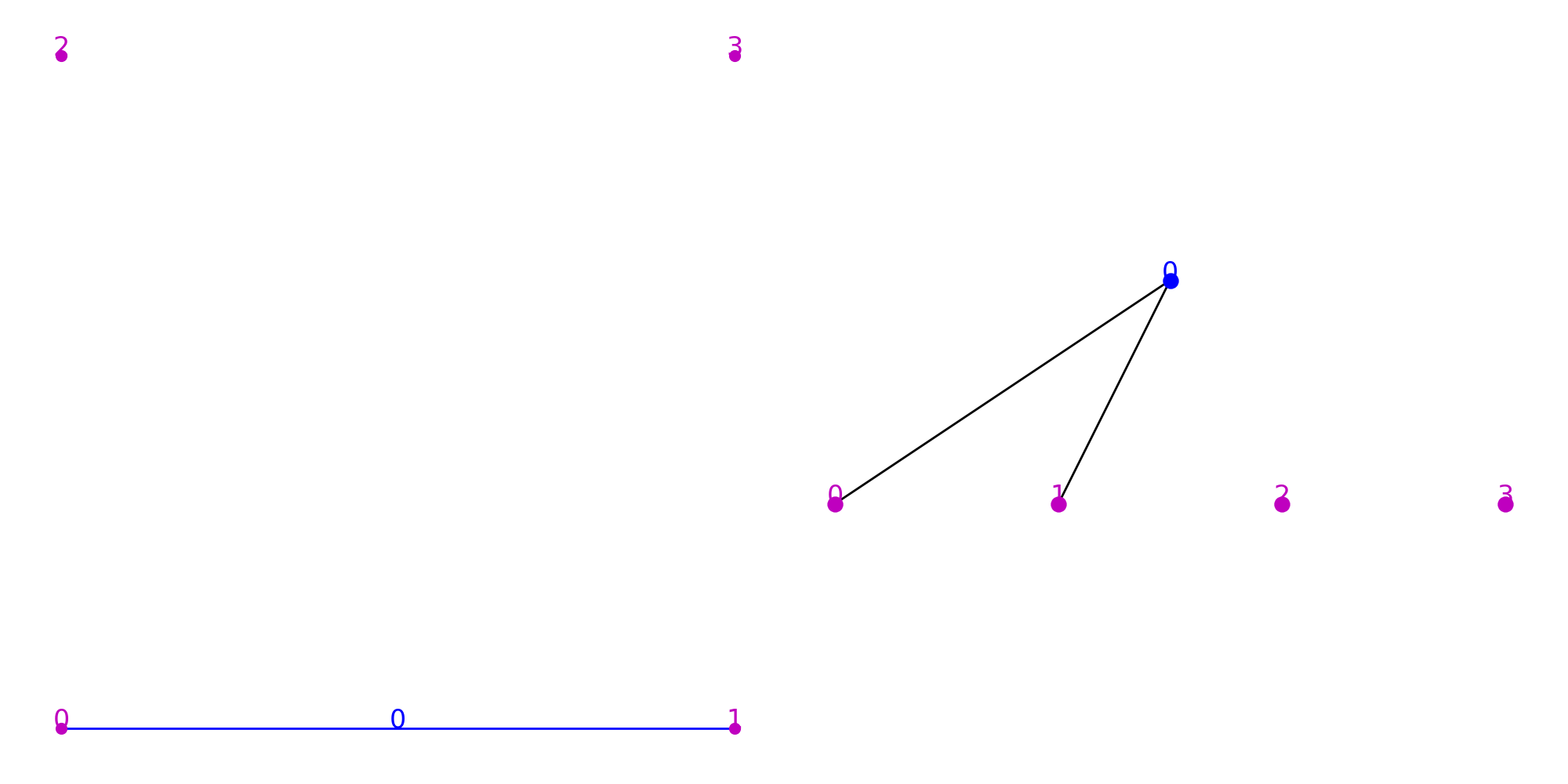
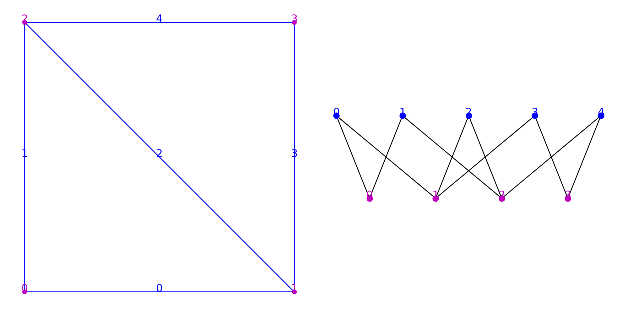
The link method allows to define the boundary relationships by assigning to the id of a wisp of dimension d the id of a wisp of dimension d-1 that forms its boundary. Let’s first add a new wisp of dimension 1 and then link it to two wisps of dimension 0 in order to create an edge.
1 2 3 | eid = topomesh.add_wisp(1)
topomesh.link(1,eid,0)
topomesh.link(1,eid,1)
|
(Source code, png, hires.png, pdf)
The basic method that allows to access the boundary relationship of a cell complex is the method borders that inputs a dimension and a wisp ID and yields the list of all wisp IDs of immediately inferior dimension that form the boundary of the considered element. Obviously, the method raises an error when the dimension is equal to 0. For example this call lists the vertex IDs that form the boundary of the edge element (dimension 1) of ID 0.
1 | print(list(topomesh.borders(1,0)))
|
[0, 1]
To complete the topological structure, one must explicitly add all the necessary elements and call link so that all necessary connections are made.
Note
For the structure to be valid, all the wisps of dimension 1 should have 2 borders of dimenson 0.
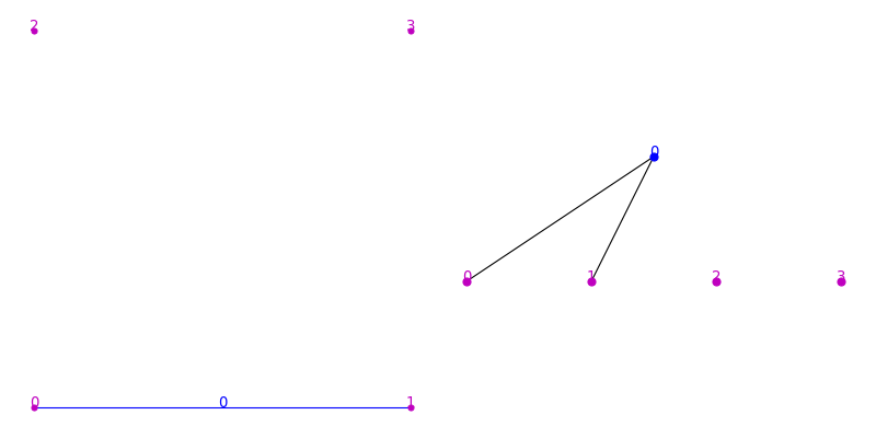
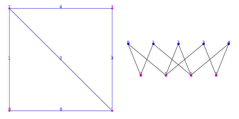
1 2 3 4 5 6 7 8 9 10 11 12 13 | topomesh.add_wisp(1,1)
topomesh.add_wisp(1,2)
topomesh.add_wisp(1,3)
topomesh.add_wisp(1,4)
topomesh.link(1,1,0)
topomesh.link(1,1,2)
topomesh.link(1,2,1)
topomesh.link(1,2,2)
topomesh.link(1,3,1)
topomesh.link(1,3,3)
topomesh.link(1,4,2)
topomesh.link(1,4,3)
|
(Source code, png, hires.png, pdf)
At this state, the complex is only formed by a collection of edges and vertices. To create faces, we have to add new elements of dimension 2, and link them to the edges that define their boundaries. In the same way, to create a cell element, we have to create a wisp of topological dimension 3 and define the set of faces that constitute its boundary.
Note
Unlike several other mesh representations, the link between faces and their vertices is not direct. It is only through the boundary relationship between faces and edges and between edges and vertices that we can access the vertices of a face.
1 2 3 4 5 6 7 8 9 10 11 12 13 14 | topomesh.add_wisp(2,0)
topomesh.add_wisp(2,1)
topomesh.link(2,0,0)
topomesh.link(2,0,1)
topomesh.link(2,0,2)
topomesh.link(2,1,2)
topomesh.link(2,1,3)
topomesh.link(2,1,4)
topomesh.add_wisp(3,0)
topomesh.link(3,0,0)
topomesh.link(3,0,1)
|
(Source code, png, hires.png, pdf)
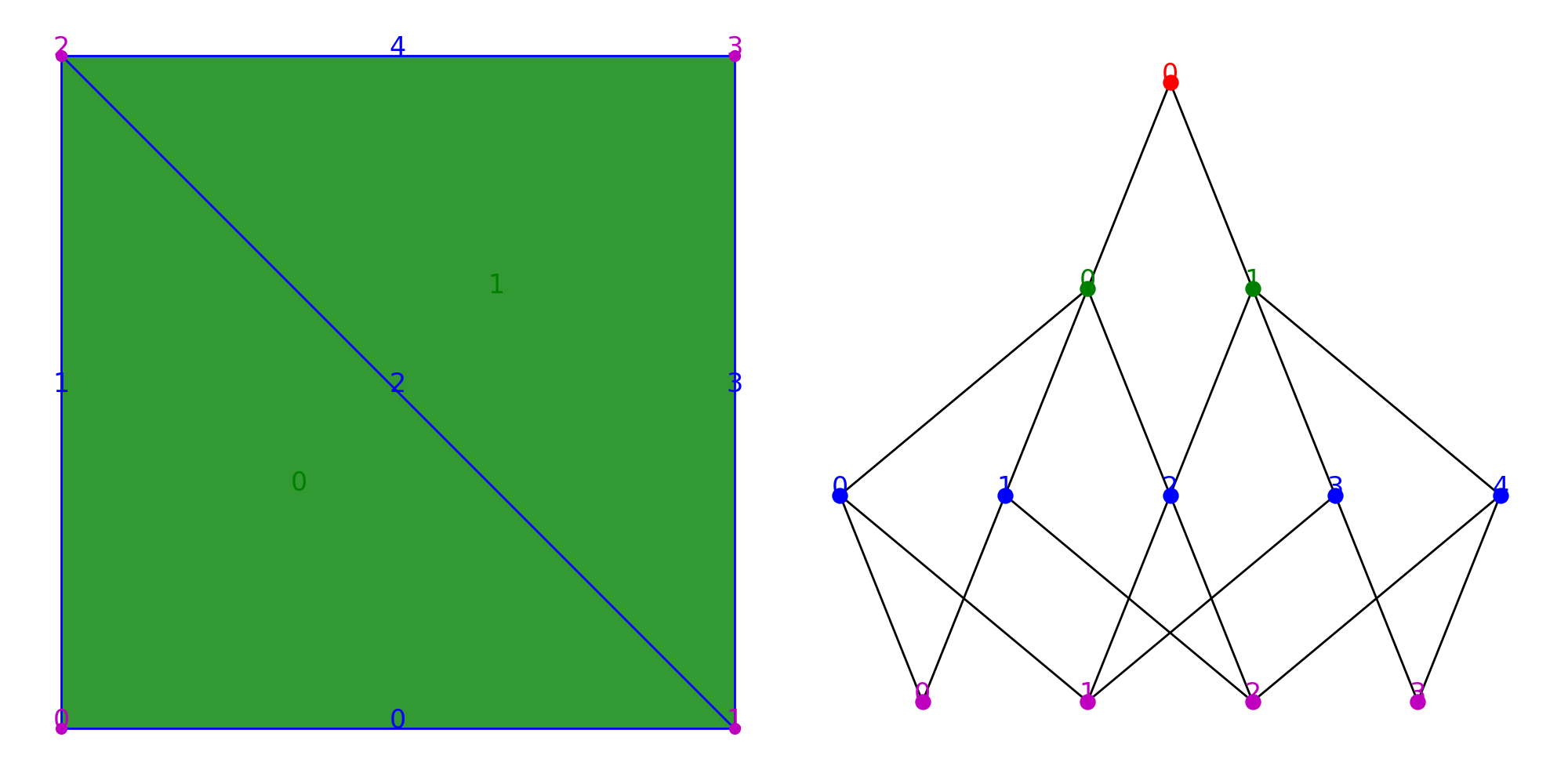
Conversely to the borders method, the regions method makes it possible to access the IDs of the wisps of which a given wisp is a boundary. The method can not be called on wisps of highest dimension (in that case 3). Here for instance, the edge 0 only has one region, the triangular face with ID 0, whereas the edge 2 has two, faces 0 and 1.
1 2 | print(list(topomesh.regions(1,0)))
print(list(topomesh.regions(1,2)))
|
[0]
[0, 1]
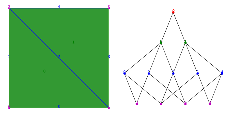
Both the regions and borders methods may take a third argument that represent the offset of the relationship. The borders of a wisp of dimension d with an offset o are the wisps of dimension d-o that are part of its boundary (respectively d+o for the regions).
1 | print(list(topomesh.borders(2,0,2)))
|
[0, 1, 2]
The construction of a complex PropertyTopomesh using these primitives is a tedious task. Fortunately, CellComplex comes with a number of pre-built functions to facilitate the construction of complexes, but all of them rely on the methods add_wisp and link to build the complex. Some examples can be found in Creation. In any case, the borders and regions methods are very useful tools to perform traversals on a cell complex.
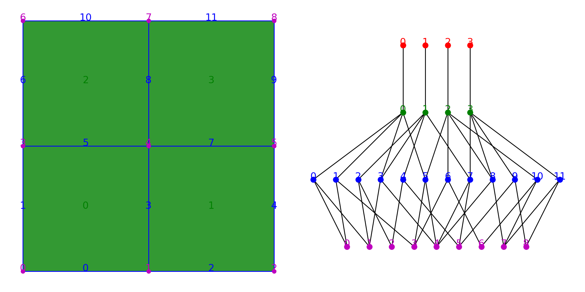
Neighbor relationship(s)
The incidence relationship accessible through regions and borders makes a connection between elements of different topological dimensions. However, it is often useful to look for elements of the same dimension that are adjacent to each other. This is what the neighbor relationship is about.
But whether two wisps of a given dimension can be considered neighbors is not necessarily uniquely defined. In the case of dimension 0 for instance, we generally consider two vertices to be neighbors if they are linked together by an edge (i.e. an element of dimension 1). This corresponds to the concept of region_neighbors where the neighborhood relationship is defined as the borders of the regions. In other terms, it requires going up one level in the incidence graph before going down one level to link two elements.
1 2 3 4 5 | from cellcomplex.property_topomesh.example_topomesh import square_grid_topomesh
topomesh = square_grid_topomesh(1)
print(list(topomesh.region_neighbors(0,3)))
|
[0, 4, 6]
(Source code, png, hires.png, pdf)
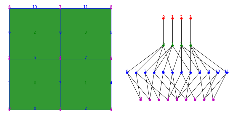
However if we apply the same logic to edges, or even faces the results might be surprising. For instance here, all the faces have 0 region_neighbors, since each face corresponds to a unique cell at dimension 3. They don’t have shared regions, so they don’t have neighbors defined by their common regions.
1 2 | for f in topomesh.wisps(2):
print("Face "+str(f)+": "+str(topomesh.nb_region_neighbors(2,0))+" neighbors")
|
Face 0: 0 neighbors
Face 1: 0 neighbors
Face 2: 0 neighbors
Face 3: 0 neighbors
In this case, it is more appropriate to look for the wisps of the same dimension that have at least one border in common with the considered wisp. In other terms, to go down one level in the incidence graph before going up one level to connect two neighbors. This is what the border_neighbors method does.
1 | print(list(topomesh.border_neighbors(2,0)))
|
[1, 2]
Note
If you wanted to find the faces that share at least one vertex with the considered face, you would need to go one level further in the adjacency graph. This offset functionality is not supported in the region_neighbors and border_neighbors methods.
Neighbor relationships are implicitly contained in the incidence graph structure that is at the core of PropertyTopomesh, but it requires a small computation at each call. Instead, it might be more efficient to pre-compute all neighbors once to perform more efficiently. The way to do it is illustrated along with other tools to simplify topology-based computations in the Topology Analysis example page
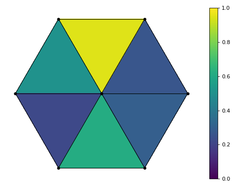
Properties
The data structure contains the geometry and topology of the cells of the complex, and also offers the possibility to assign any number of properties to each of its topological elements (vertices, edges, faces or cells) under the form of dictionaries pairing wisp IDs and property values.
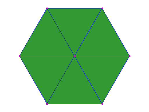
The following code assigns a new scalar property to faces. The method update_wisp_property inputs a property name, a dimension and a dictionary and in this case assigns a random value (between 0 and 1) to each face element of the hexagon cellcomplex.
1 2 3 4 5 6 | import numpy as np
from cellcomplex.property_topomesh.example_topomesh import hexagon_topomesh

topomesh = hexagon_topomesh()
topomesh.update_wisp_property('random',2,dict(zip(topomesh.wisps(2),np.random.rand(topomesh.nb_wisps(2)))))
|
(Source code, png, hires.png, pdf)
Note
Properties can be of any type, however it is recommended that for a given property, all wisps share the same property type.
- The functions in
CellComplexwill generally support:
The method wisp_property returns an array_dict instance that makes it possible to modify the values stored in the structure, using the IDs of the wisps as keys of the dictionary.
1 2 3 | for w in topomesh.wisps(2):
topomesh.wisp_property('random',2)[w] = 1
print(topomesh.wisp_property('random',2))
|
{0: 1.0,
 1: 1.0,
 2: 1.0,
 3: 1.0,
 4: 1.0,
 5: 1.0}
Properties are useful to store a number of useful data on the topological elements of the complex, for instance topological information that we don’t want to recompute (neighbor IDs, face vertices,…) of geometrical information that can be computed using topology and vertex positions. There is a whole module named property_topomesh_analysis that provides tools to compute useful properties on cell complexes. Most of them are presented in the Geometry Analysis example page of this documentation.